Creating Physiological Bounds

To make crnt4sbml more user friendly and make its search limited to physiological problems, we have constructed the functions crnt4sbml.MassConservationApproach.get_optimization_bounds() and crnt4sbml.SemiDiffusiveApproach.get_optimization_bounds(), which constructs the appropriate bounds that must be provided to the mass conservation and semi-diffusive optimization routines, respectively. Although this feature can be extremely useful especially if the user is continually changing the SBML file, it should be used with some amount of caution.

Preprocessing

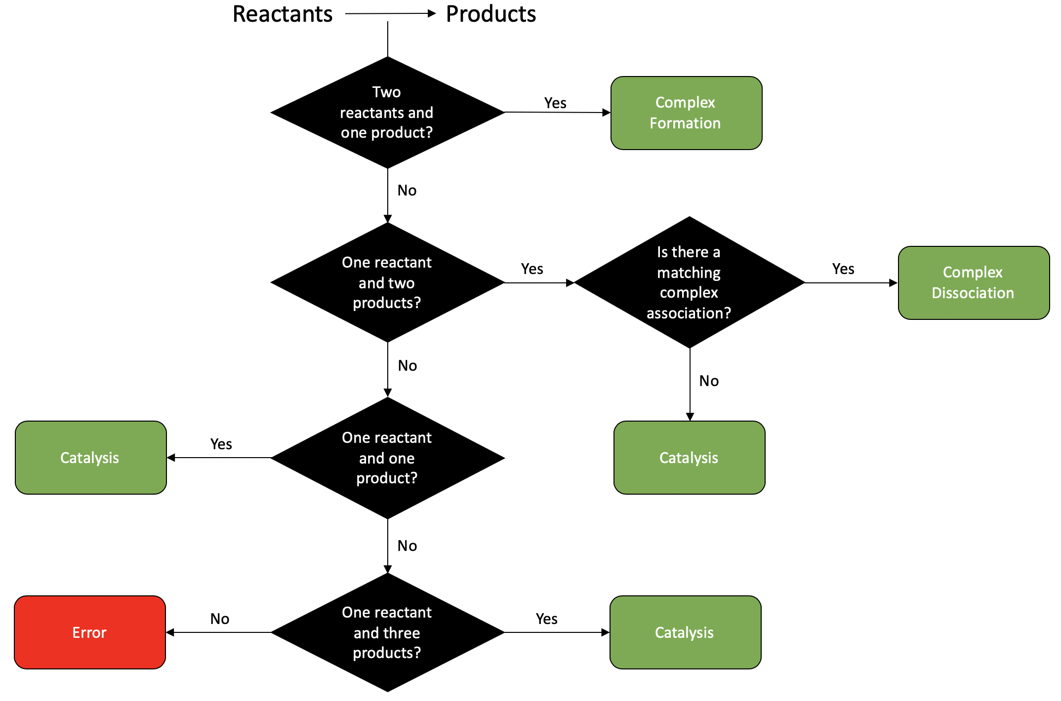
To provide these physiological bounds, crnt4sbml first identifies the reactions of the network. A reaction can be identified as complex formation, complex dissociation, or catalysis, no other type of reaction is considered. To make this assignment, the reactants and products of the reaction along with the associated stoichiometries are found for the particular reaction. Using the sum of the stoichiometries for the reactants and products the decision tree below is used to determine the type of reaction. If the reaction is not identified as complex formation, complex dissociation, or catalysis, then an error message will be provided and the reaction type will be specified as “None”.

The type of reaction assigned by crnt4sbml can always be found by running the following script where we let Fig1Ci.xml be our SBML file

import crnt4sbml
network = crnt4sbml.CRNT("/path/to/Fig1Ci.xml")
network.print_biological_reaction_types()

this provides the output below:

Reaction graph of the form
reaction -- reaction label -- biological reaction type:
s1+s2 -> s3  --  re1 -- complex formation
s3 -> s1+s2  --  re1r -- complex dissociation
s3 -> s6+s2  --  re2 -- catalysis
s6+s7 -> s16  --  re3 -- complex formation
s16 -> s6+s7  --  re3r -- complex dissociation
s16 -> s7+s1  --  re4 -- catalysis
s1+s6 -> s15  --  re5 -- complex formation
s15 -> s1+s6  --  re5r -- complex dissociation
s15 -> 2*s6  --  re6 -- catalysis

Creating the proper constraints for the optimization routine for the mass conservation approach differs from that of the semi-diffusive approach. This is because the mass conservation approach requires bounds for the rate constants and species’ concentrations while the semi-diffusive approach only requires bounds for the fluxes of the reactions.

Mass Conservation Approach

To construct physiological bounds for the rate constants we first identify the type of the reaction and then we use the function crnt4sbml.CRNT.get_physiological_range(), which provides a tuple corresponding to the lower and upper bounds. The values for these bounds are in picomolar (pM). Here we assign pM values rather than molar values because these values are larger and tend to make running the optimization routine much easier. In molar ranges or values close to zero, the optimization becomes difficult because the routine is attempting to minimize an objective function which has a known value of zero. Thus, if the user wishes to assign different bounds, it is suggested that these bounds be scaled such that they are not close to zero.

We now demonstrate the physiological bounds produced for the SBML file Fig1Ci.xml

import crnt4sbml
network = crnt4sbml.CRNT("/path/to/Fig1Ci.xml")

approach = network.get_mass_conservation_approach()

bounds, concentration_bounds = approach.get_optimization_bounds()

print(bounds)

print(concentration_bounds)

this provides the following output:

Creating Equilibrium Manifold ...
Elapsed time for creating Equilibrium Manifold: 2.060944

[(1e-08, 0.0001), (1e-05, 0.001), (0.001, 1.0), (1e-08, 0.0001), (1e-05, 0.001), (0.001, 1.0), (1e-08, 0.0001), (1e-05, 0.001), (0.001, 1.0), (0.5, 500000.0), (0.5, 500000.0), (0.5, 500000.0)]
[(0.5, 500000.0), (0.5, 500000.0), (0.5, 500000.0), (0.5, 500000.0)]

Where the rate constants and species’ concentrations for the list “bounds” can be found by the following command

print(approach.get_decision_vector())

providing the output:

[re1, re1r, re2, re3, re3r, re4, re5, re5r, re6, s2, s6, s15]

and the species’ concentrations referred to in the list “concentration_bounds” can be determined by the following

print(approach.get_concentration_bounds_species())

giving the output:

[s1, s3, s7, s16]

Semi-diffusive Approach

As stated above, the semi-diffusive approach only requires bounds for the fluxes of the reactions. To assign these values, we again use the function crnt4sbml.CRNT.get_physiological_range(), which provides a tuple for the lower and upper bounds. However, the values returned by this call are given in molars. The unit of molars is suggested because the ranges produced for fluxes are much smaller than those for pM, making the optimization easier.

To demonstrate the bounds produced for the semi-diffusive approach, we use the SBML file Fig1Cii.xml.

import crnt4sbml
network = crnt4sbml.CRNT("/path/to/Fig1Cii.xml")

approach = network.get_semi_diffusive_approach()

bounds = approach.get_optimization_bounds()

print(bounds)

this provides the following output:

[(0, 55), (0, 55), (0, 55), (0, 55), (0, 55), (0, 55), (0, 55), (0, 55), (0, 55), (0, 55), (0, 55), (0, 55)]

the elements of which correspond to the fluxes that can be obtained from the following command

approach.print_decision_vector()

which provides the output:

Decision vector for optimization:
[v_2, v_3, v_4, v_5, v_6, v_7, v_9, v_11, v_13, v_15, v_17, v_18]

Reaction labels for decision vector:
['re1r', 're3', 're3r', 're6', 're6r', 're2', 're8', 're17r', 're18r', 're19r', 're21', 're22']

Here the decision vector for optimization is defined in terms of fluxes of the reactions. To make identifying which flux we are considering easier, the command above relates the flux to the reaction label. Thus, flux ‘v_2’ refers to the flux of reaction ‘re1r’.