Direct Simulation for the General Approach

When using the general approach it is possible that the optimization routine finds kinetic constants that force the Jacobian of the system to be ill-conditioned or even singular, even if species concentrations are varied. If this particular scenario occurs, numerical continuation will not be able to continue as it relies on a well-conditioned Jacobian. To overcome this type of situation we have constructed the function crnt4sbml.GeneralApproach.run_direct_simulation() for the general approach. The direct simulation routine strategically chooses the initial conditions for the ODE system and then simulates the ODEs until a steady state occurs. Then based on the user defined signal and optimization values provided, it will vary the signal amount and simulate the ODE system again until a steady state occurs. By varying the signal for several values and different initial conditions, direct simulation is able to construct a bifurcation diagram. Given the direct simulation method is numerically integrating the system of ODEs, this method will often take longer than the numerical continuation routine. Although this is the case, direct simulation may be able to provide a bifurcation diagram when numerical continuation cannot.

Failure of numerical continuation

In the following example we consider the case where numerical continuation fails to provide the appropriate results. For this example, we will be using the SBML file simple_biterminal.xml. We then construct the following script, where we are printing the output of the numerical continuation.

import crnt4sbml
network = crnt4sbml.CRNT("/path/to/simple_biterminal.xml")
signal = "C2"
response = "s11"
bnds = [(2.4, 2.42), (27.5, 28.1), (2.0, 2.15), (48.25, 48.4), (0.5, 1.1), (1.8, 2.1), (17.0, 17.5), (92.4, 92.6),
        (0.01, 0.025), (0.2, 0.25), (0.78, 0.79), (3.6, 3.7), (0.15, 0.25), (0.06, 0.065)] + \ [(0.0, 100.0),
        (18.0, 18.5), (0.0, 100.0), (0.0, 100.0), (27.0, 27.1), (8.2, 8.3), (90.0, 90.1), (97.5, 97.9), (30.0, 30.1)]

approach = network.get_general_approach()
approach.initialize_general_approach(signal=signal, response=response)

params_for_global_min, obj_fun_vals = approach.run_optimization(bounds=bnds, iterations=15, dual_annealing_iters=1000,
                                                                confidence_level_flag=True, parallel_flag=False)

multistable_param_ind, plot_specifications = approach.run_greedy_continuity_analysis(species=response, parameters=params_for_global_min, print_lbls_flag=True,
                                                                                     auto_parameters={'PrincipalContinuationParameter': signal})
approach.generate_report()

This provides the following output:

Running the multistart optimization method ...
Elapsed time for multistart method: 2590.524824142456

It was found that 2.1292329042333798e-16 is the minimum objective function value with a confidence level of 0.680672268907563 .
1 point(s) passed the optimization criteria.

Running continuity analysis ...
J0: -> s11; re7c*s2s10 - re8*s11;J1: -> s2; -re1*s2*(C2 - s2 - s2s10 - s2s9 - 2.0*s3 - 2.0*s6) + re1r*s3 -
re2*s2*(C2 - s2 - s2s10 - s2s9 - 2.0*s3 - 2.0*s6) + re2r*s6 + 2*re4*s6 + re5c*s2s9 + re5d*s2s9 -
re5f*s2*(C1 - s10 - s11 - s2s10 - s2s9) + re7c*s2s10 + re7d*s2s10 - re7f*s10*s2;
J2: -> s3; re1*s2*(C2 - s2 - s2s10 - s2s9 - 2.0*s3 - 2.0*s6) - re1r*s3 - re3*s3;
J3: -> s6; re2*s2*(C2 - s2 - s2s10 - s2s9 - 2.0*s3 - 2.0*s6) - re2r*s6 - re4*s6;
J4: -> s10; re5c*s2s9 - re6*s10 + re7d*s2s10 - re7f*s10*s2 + re8*s11;
J5: -> s2s9; -re5c*s2s9 - re5d*s2s9 + re5f*s2*(C1 - s10 - s11 - s2s10 - s2s9);
J6: -> s2s10; -re7c*s2s10 - re7d*s2s10 + re7f*s10*s2;
re1 = 2.4179937298574217;re1r = 27.963833386686552;re2 = 2.1212280827699264;re2r = 48.342142632557824;
re3 = 0.9103403848297675;re4 = 1.8021182302742345;re5f = 17.01982705623611;re5d = 92.47396549104621;
re5c = 0.021611755555125196;re6 = 0.23540156485799416;re7f = 0.7824887292735982;re7d = 3.692336204373193;
re7c = 0.20574339517454907;re8 = 0.06329703678602935;s1 = 14.749224746318406;s2 = 18.117522179242442;
s3 = 22.37760479141668;s6 = 11.304051540693258;s9 = 27.001718858136442;s10 = 8.264281271233568;
s2s9 = 90.01696959750683;s11 = 97.69532935525308;s2s10 = 30.05600671002251;C1 = 253.03430579215245;C2 = 220.30303589731005;
Labels from numerical continuation:
['EP', 'MX']
Labels from numerical continuation:
['EP', 'MX']
Labels from numerical continuation:
['EP', 'MX']
Labels from numerical continuation:
['EP', 'MX']
Labels from numerical continuation:
['EP', 'MX']
Labels from numerical continuation:
['EP', 'MX']
Labels from numerical continuation:
['EP', 'MX']
Labels from numerical continuation:
['EP', 'MX']
Labels from numerical continuation:
['EP', 'MX']
Labels from numerical continuation:
['EP', 'MX']

Elapsed time for continuity analysis in seconds: 4.751797914505005

Number of multistability plots found: 0
Elements in params_for_global_min that produce multistability:
[]

As we can see, the numerical continuation is unable to find limit points for the example. This is due to the Jacobian being ill-conditioned. In cases where the output of the numerical continuation is consistently “[‘EP’, ‘MX’]” or one of the points is “MX”, this often indicates that the Jacobian is ill-conditioned or always singular. If this situation is encountered, it is suggested that the user run the direct simulation routine.

Outline of direct simulation process

To cover the corner case where numerical continuation is unable to complete because the Jacobian is ill-conditioned, we have constructed a direct simulation approach. This approach directly simulates the full ODE system for the network by numerically integrating the ODE system. Using these results, a bifurcation diagram is then produced. In the following subsections we will provide an overview of the workflow carried out by the direct simulation method.

Finding the appropriate initial conditions

When numerically integrating the full system of ODEs we use the SciPy routine solve_ivp. This routine solves an initial value problem for a system of ODEs. For this reason, we need to provide initial conditions that correspond to the optimization values provided. We need to do this for two cases, one where we obtain a high concentration of the response species and another where we obtain a lower concentration of the response species, at a steady state. To do this we use the first element of the optimization values provided to the routine (which correspond to an input vector consisting of reaction constants and species concentrations) to calculate the conservation laws for the problem.

Once we have the conservation law values, we then construct construct all possible initial conditions for the ODE system. This is done by using the conservation laws of the problem. For our example, we have the following conservation laws:

C1 = 1.0*s10 + 1.0*s11 + 1.0*s2s10 + 1.0*s2s9 + 1.0*s9
C2 = 1.0*s1 + 1.0*s2 + 1.0*s2s10 + 1.0*s2s9 + 2.0*s3 + 2.0*s6

Thus, we can put the total C1 value in any of the following species: s10, s11, s2s10, s2s9, or s9, in addition to this, we can put the total C2 value in any of the following species: s1, s2, s2s10, s2s9, s3, or s6. For example, we can set the initial condition for the system by setting the initial value of s10 = C1, s1 = C2, and all other species to zero. As one can see, we need to test all possible combinations of these species to see the set that appropriately corresponds to the optimization values provided. The number of combinations tested can be reduced by removing duplicate combinations and repeated species.

To determine the combination that we will use to conduct the bistability analysis, we first find the steady state (using the process outlined in the next subsection) for the corresponding initial condition. Using these steady state values, we then determine the conservation law values at the steady state. If the conservation law values align with the conservation law values calculated using the first element of the optimization values, then we consider this combination as a viable combination. Once we have all of the viable combinations, we then select a set of two of these combinations, where one produces a high concentration of the response species and the other has a lower concentration of the response species, at the steady state. To see the initial conditions that will be used for the bistability analysis, one can set print_flag=True in crnt4sbml.GeneralApproach.run_direct_simulation(). This provides the following output for the example:

For the forward scan the following initial condition will be used:
s1 = 0.0
s2 = C2
s3 = 0.0
s6 = 0.0
s9 = 0.0
s10 = C1
s2s9 = 0.0
s11 = 0.0
s2s10 = 0.0

For the reverse scan the following initial condition will be used:
s1 = 0.0
s2 = C2
s3 = 0.0
s6 = 0.0
s9 = C1
s10 = 0.0
s2s9 = 0.0
s11 = 0.0
s2s10 = 0.0

The process of finding these viable combinations can take a long time depending on the network provided. For this reason, this process can be done in parallel by setting parallel_flag=True in crnt4sbml.GeneralApproach.run_direct_simulation(). For more information on parallel runs refer to Parallel CRNT4SBML.

Finding a steady state to the system

In order to produce a bifurcation diagram, we need to consider the solution of the system of ODEs at a steady state. Due to the nature of the system of ODEs, this solution is often to complex to find analytically. For this reason, we find this solution by numerically integrating the system until we reach a steady state in the system. As mentioned previously, this is done by using the Scipy routine solve_ivp. Specifically, we utilize the BDF method with a rtol of 1e-6 and a atol of 1e-9. To begin, we start with an interval of integration of 0.0 to 100.0, we then continue in increments of 100 until a steady state has been reached or 1000 increments have been completed. A system of ODEs is considered to be at a steady state when the relative error (of the last and current time step of the concentration of the response species) is less than or equal to the user defined variable change_in_relative_error of crnt4sbml.GeneralApproach.run_direct_simulation(). It should be noted that a smaller value of change_in_relative_error will run faster, but may produce an ODE system that is not at a steady state.

Constructing the bifurcation diagram

Once the appropriate initial conditions have been given, the direct simulation routine then attempts to construct a bifurcation diagram. Note that this process does not guarantee that a bifurcation diagram with bistability will be provided, rather it will produce a plot of the long-term behavior of the ODEs in a particular interval for the user defined signal. The first step in this process is defining the search radius of the signal. This search radius can be defined by the user by modifying the variables left_multiplier and right_multiplier of crnt4sbml.GeneralApproach.run_direct_simulation(), which provide a lower and upper -bound for the signal value. Specifically, when considering different values of the signal, the range for these different values will be in the interval [signal_value - signal_value*left_multiplier, signal_value - signal_value*right_multiplier], where the signal value is the beginning value of the signal as provided by the input vectors produced by optimization.

Using this range, the routine then splits the range into 100 evenly spaced numbers. The signal is then set equal to each of these numbers and the ODE system is simulated until a steady state occurs, using the initial conditions of both the forward and reverse scan values established in the previous subsection. Using all 200 values, the minimum and maximum value of the response species’ concentration is found. This process is then repeated using 60 evenly spaced numbers between the signal values that correspond to the minimum and maximum values of the response species’ concentration. Using the 120 values produced, the minimum and maximum values of the response species are found. This process is repeated for 5 iterations or until there are 10 or more signal values between the signal values that correspond to the minimum and maximum values of the response species’ concentration of the current iteration. This process effectively detects and “zooms in” on the region where bistability is thought to exist. Although this process can be very effective, it can take a long time to complete. Thus, it is suggested that this be done in parallel by setting parallel_flag=True in crnt4sbml.GeneralApproach.run_direct_simulation(). 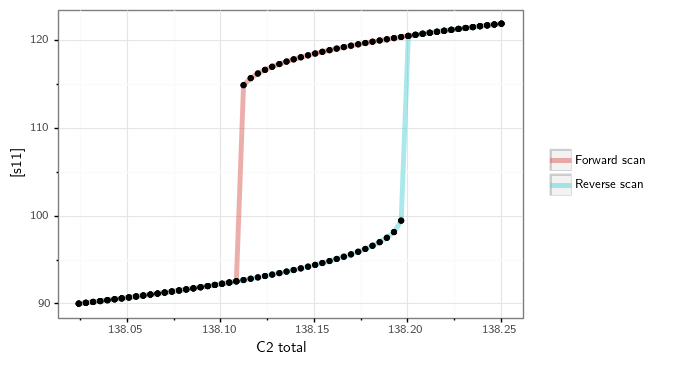For more information on parallel runs refer to Parallel CRNT4SBML. For the example we have been considering, we obtain the following bifurcation diagram.