General Approach Walkthrough
Using the SBML file constructed as in CellDesigner Walkthrough, we will proceed by completing a more in-depth
explanation of running the general approach. Note that the general approach can
be ran on any network that has conservation laws, even if that network does have a sink/source. One can test whether or
not there are conservation laws by seeing if the output of crnt4sbml.Cgraph.get_dim_equilibrium_manifold() is
greater than zero. This tutorial will use simple_biterminal.xml.
The following code will import crnt4sbml and the SBML file. For a little more detail on this process consider Low Deficiency Approach.
import crnt4sbml
network = crnt4sbml.CRNT("/path/to/simple_biterminal.xml")
If we then want to conduct the general approach, we must first initialize the general_approach, which is done as follows:
approach = network.get_general_approach()
Now that we have initialized the class, we have to tell the routine the values of the signal (or principal continuation parameter) and response of the bifurcation diagram, as well as whether or not we would like to force a steady state. Just as in Mass Conservation Approach Walkthrough, the signal (or PCP for numerical continuation) is a conservation law. To select the signal one needs to know which conservation law to choose. The following command will provide the conservation laws derived by the initialization of the general approach class:
print(approach.get_conservation_laws())
This provides the following output:
C1 = 1.0*s10 + 1.0*s11 + 1.0*s2s10 + 1.0*s2s9 + 1.0*s9
C2 = 1.0*s1 + 1.0*s2 + 1.0*s2s10 + 1.0*s2s9 + 2.0*s3 + 2.0*s6
The response of the bifurcation diagram can then be chosen as any species. For this particular example we will choose the following signal and response:
signal = "C2"
response = "s11"
Now that we have the bifurcation parameters, we should consider whether or not we would like to force a steady state in the
ODE system formed by the network by fixing the reactions. Although forcing a steady state by fixing the reactions can provide
faster results for some networks when running optimization, it does restrict the solutions found to a particular
solution, rather than looking for a general solution. If reactions are fixed, the reactions that are fixed can by found
by using crnt4sbml.GeneralApproach.get_fixed_reactions(), where the symbolic expressions for these reactions are
given by crnt4sbml.GeneralApproach.get_solutions_to_fixed_reactions().
For this particular example, fixing the reactions leads to poor results. Thus, we will choose to not fix the reactions,
this is done by setting the fix_reaction variable to False in crnt4sbml.GeneralApproach.initialize_general_approach().
Now we can initialize the rest of the general approach as follows:
approach.initialize_general_approach(signal=signal, response=response, fix_reactions=False)
Now that the approach has been constructed, we can begin to define the specific information needed for the optimization routine for the general approach. One very important value that must be provided to the optimization problem are the bounds for the species and reactions. For this reason, it is useful to see the variables and the order in which they appear. To do this one can add the following command to the script:
print(approach.get_input_vector())
This provides the following output:
[re1, re1r, re2, re2r, re3, re4, re5f, re5d, re5c, re6, re7f, re7d, re7c, re8, s1, s2, s3, s6, s9, s10, s2s9, s11, s2s10]
Using the input vector provided, one can then construct the bounds which are necessary for the optimization problem by creating a list of tuples where the first element corresponds to the lower bound value of the parameter and the second element is the upper bound value of the parameter.
As creating these bounds is not initially apparent to novice users or may become cumbersome, we have created a function call that will automatically generate physiological bounds based on the C-graph. To use this functionality one can add the following code:
bnds = approach.get_optimization_bounds()
This provides the following values:
bnds = [(1e-08, 0.0001), (1e-05, 0.001), (1e-08, 0.0001), (1e-05, 0.001), (0.001, 1.0), (0.001, 1.0), (1e-08, 0.0001),
        (1e-05, 0.001), (0.001, 1.0), (0.001, 1.0), (1e-08, 0.0001), (1e-05, 0.001), (0.001, 1.0), (0.001, 1.0),
        (0.5, 500000.0), (0.5, 500000.0), (0.5, 500000.0), (0.5, 500000.0), (0.5, 500000.0), (0.5, 500000.0),
        (0.5, 500000.0), (0.5, 500000.0), (0.5, 500000.0)]
For more information and the correctness on these bounds please refer to Creating Physiological Bounds.
Although these bounds can be used for this example, they are not ideal. For this reason, we have chosen a particular set of ranges for the species and reactions based on the input vector, which is given as follows (for reference, below we have set the range for re1 to be between 2.4 and 2.42, and set the range for s2 to be between 18.0 and 18.5):
bnds = [(2.4, 2.42), (27.5, 28.1), (2.0, 2.15), (48.25, 48.4), (0.5, 1.1), (1.8, 2.1), (17.0, 17.5), (92.4, 92.6),
        (0.01, 0.025), (0.2, 0.25), (0.78, 0.79), (3.6, 3.7), (0.15, 0.25), (0.06, 0.065)] + [(0.0, 100.0),
        (18.0, 18.5), (0.0, 100.0), (0.0, 100.0), (27.0, 27.1), (8.2, 8.3), (90.0, 90.1), (97.5, 97.9), (30.0, 30.1)]
The next most important parameter for optimization is the number of initial points for the multi-start optimization. It is usually good practice to run the optimization with 100 initial points and observe the minimum objective function value achieved. If an objective function value smaller than machine epsilon is not achieved, it is best to rerun the optimization with more initial points. If 10000 or more points are used and an objective function value smaller than machine epsilon is not achieved, then it is possible that the network does not produce bistability (although this test does not exclude the possibility for bistability to exist, as stated in the theory). One can even use the built-in confidence level option as described in Confidence Level Routine to make an informed decision on whether or not to continue performing more iterations. We state the number of initial points below.
iters = 15
The last values that can be defined before the optimization portion (as provided below) are the number of iterations
allowed for the Dual Annealing optimization method used (provided by
Scipy),
the seed for the random number generation in the optimization method (below we set this to 0 so we can reproduce the
results, None should be used if we want the method to be random), and the print_flag which tells the program if the
objective function value and decision vector for the multi-start method should be printed out (here we set it to False,
which means no output will be provided). See crnt4sbml.GeneralApproach.run_optimization()
for the default values of the routine.
d_iters = 1000
sd = 0
prnt_flg = False
Using these values, we run the optimization problem using the following command, which returns a list of the parameters (which correspond to the input vector) and corresponding objective function values that produce an objective function value smaller than machine epsilon.
params_for_global_min, obj_fun_vals = approach.run_optimization(bounds=bnds, iterations=iters, seed=sd, print_flag=prnt_flg,
                                                                dual_annealing_iters=d_iters, confidence_level_flag=True)

approach.generate_report()
The following is the output obtained after running the above code:
Running the multistart optimization method ...
Elapsed time for multistart method: 2590.524824142456

It was found that 2.1292329042333798e-16 is the minimum objective function value with a confidence level of 0.680672268907563 .
1 point(s) passed the optimization criteria.
From this output, it is apparent that for some networks the optimization for the general approach can take a long time to complete. For this reason, we have a parallel version of the optimization approach. An example of a parallel general approach can be found in subsection Parallel General Approach of section Parallel CRNT4SBML.
If the optimization routine returns objective function values smaller than machine epsilon, then bistability analysis can
be conducted. As in Mass Conservation Approach Walkthrough and Semi-diffusive Approach Walkthrough this can be done by using numerical
continuation. See the functions crnt4sbml.GeneralApproach.run_continuity_analysis() and
crnt4sbml.GeneralApproach.run_greedy_continuity_analysis() for more information on using numerical continuation with
the general approach. Although numerical continuation can be used by most examples, in some cases, the input vectors
found by the optimization method yield an ODE system that has a singular or ill-conditioned Jacobian. For this reason,
the numerical continuation method will be unsuccessful. In the simple_biterminal example, this is what occurs. To provide
an alternative method to numerical continuation, we have constructed a routine that performs direct simulation in order
to construct the bifurcation diagram. See section Direct Simulation for the General Approach for further information on the method.
To run bistability analysis using the direct simulation approach, we run the following routine:
approach.run_direct_simulation(params_for_global_min)
This routine will use the input vectors (named params_for_global_min) provided by the optimization and perform the direct simulation approach for bistability analysis, then puts the plots produced in the directory path ./dir_sim_graphs. This provides the following output for the simple_biterminal example:
Starting direct simulation ...
Elapsed time for direct simulation in seconds: 189.25777792930603
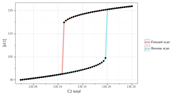
Along with this, it also produces the following bifurcation diagram.
Similar to the optimization for the general approach, we can see that direct simulation can take a long time to complete. For this reason, we have a parallel version of the direct simulation approach. An example of a parallel direct simulation run for the general approach can be found in subsection Parallel General Approach of section Parallel CRNT4SBML.
For more examples of running the general approach please see Further Examples.