Semi-diffusive Approach Walkthrough
Using the SBML file constructed as in CellDesigner Walkthrough, we will proceed by completing a more in-depth
explanation of running the semi-diffusive approach of [OMYS17]. This tutorial will use the SBML file
Fig1Cii.xml. The following code will
import crnt4sbml and the SBML file. For a little more detail on this process consider Low Deficiency Approach.
import crnt4sbml
network = crnt4sbml.CRNT("/path/to/Fig1Cii.xml")
If we then want to conduct the semi-diffusive approach of [OMYS17], we must first initialize the semi_diffusive_approach, which is done as follows:
approach = network.get_semi_diffusive_approach()
This command creates all the necessary information to construct the optimization problem to be solved. Unlike the mass conservation approach, there should be no output provided by this initialization. Note that if a boundary species is not provided or there are conservation laws present, then the semi-diffusive approach will not be able to be ran. If conservation laws are found, then the mass conservation approach should be ran.
As in the mass conservation approach, it is very important to view the decision vector constructed for the optimization routine. In the semi-diffusive approach, the decision vector produced is in terms of the fluxes of the reactions. To make the decision vector more clear, the following command will print out the decision vector and also the corresponding reaction labels.
approach.print_decision_vector()
This provides the following output:
Decision vector for optimization:
[v_2, v_3, v_4, v_5, v_6, v_7, v_9, v_11, v_13, v_15, v_17, v_18]

Reaction labels for decision vector:
['re1r', 're3', 're3r', 're6', 're6r', 're2', 're8', 're17r', 're18r', 're19r', 're21', 're22']
As in the mass conservation approach, if your are using an SBML file you created yourself, the output may differ. If you would like an explicit list of the decision vector you can use the following command:
print(approach.get_decision_vector())
Using the decision vector as a reference, we can now provide the bounds for the optimization routine. As creating these bounds is not initially apparent to novice users or may become cumbersome, we have created a function call that will automatically generate physiological bounds based on the C-graph. To use this functionality one can add the following code:
bounds = approach.get_optimization_bounds()
This provides the following values:
bounds = [(0, 55), (0, 55), (0, 55), (0, 55), (0, 55), (0, 55), (0, 55), (0, 55), (0, 55), (0, 55), (0, 55), (0, 55)]
For more information and the correctness on these bounds please refer to Creating Physiological Bounds. An important check that should be completed for the semi-diffusive approach is to verify that that the key species, non key species, and boundary species are correct. This can be done after initializing the semi-diffusive approach as follows:
print(approach.get_key_species())
print(approach.get_non_key_species())
print(approach.get_boundary_species())
This provides the following results for our example:
['s1', 's2', 's7']

['s3', 's6', 's8', 's11']

['s21']
Using this information, we can now run the optimization in a similar manner to the mass conservation approach. First we will
initialize some variables for demonstration purposes. In practice, the user should only need to define the bounds and
number of iterations to run the optimization routine. For more information on the defaults of the optimization routine,
see crnt4sbml.SemiDiffusiveApproach.run_optimization().
import numpy
num_itr = 100
sys_min = numpy.finfo(float).eps
sd = 0
prnt_flg = False
num_dtype = numpy.float64
We now run the optimization routine for the semi-diffusive approach:
params_for_global_min, obj_fun_val_for_params = approach.run_optimization(bounds=bounds, iterations=num_itr, seed=sd,
                                                                          print_flag=prnt_flg, numpy_dtype=num_dtype,
                                                                          sys_min_val=sys_min)
The following is the output obtained by the constructed model:
Running feasible point method for 100 iterations ...
Elapsed time for feasible point method: 1.542820930480957

Running the multistart optimization method ...
Elapsed time for multistart method: 184.3005211353302
For a detailed description of the optimization routine see Numerical Optimization Routine. At this point it may also be helpful to generate a report on the optimization routine that provides more information. To do this execute the following command:
approach.generate_report()
This provides the following output:
Smallest value achieved by objective function: 0.0
76 point(s) passed the optimization criteria.
The first line tells the user the smallest value that was achieved after all of the iterations have been completed. The next line tells one the number of feasible points that produce an objective function value smaller than sys_min_val that also pass all of the constraints of the optimization problem. Given the optimization may take a long time to complete, it may be important to save the parameters produced by the optimization. This can be done as follows:
numpy.save('params.npy', params_for_global_min)
this saves the list of numpy arrays representing the parameters into the npy file params. The user can then load these values at a later time by using the following command:
params_for_global_min = numpy.load('params.npy')
Similar to the mass conservation approach, we can run numerical continuation for the semi-diffusive approach. Note that the principal continuation parameter (PCP) now corresponds to a reaction rather than a constant as in the mass conservation approach. However, the actual continuation will be performed with respect to the flux of the reaction. The y-axis of the continuation can then be set by defining the species, here we choose the species s7. For the semi-diffusive network we conduct the numerical continuation for the semi-diffusive approach as follows:
multistable_param_ind, plot_specifications = approach.run_continuity_analysis(species='s7', parameters=params_for_global_min,
                                                                              auto_parameters={'PrincipalContinuationParameter': 're17',
                                                                                               'RL0': 0.1, 'RL1': 100, 'A0': 0.0,
                                                                                                'A1': 10000})
In addition to putting the multistability plots found into the folder num_cont_graphs, this routine will also return the indices of params_for_global_min that correspond to these plots named “multistable_param_ind” above. Along with these indices, the routine will also return the plot specifications for each element in “multistable_param_ind” that specify the range used for the x-axis, y-axis, and the x-y values for each special point in the plot (named “plot_specifications” above). Also note that if multistability plots are produced, the plot names will have the following form: PCP_species id_index of params_for_global.png. For more information on the AUTO parameters provided and the continuation routine itself, refer to Numerical Continuation Routine. This provides the following output:
Running continuity analysis ...
Elapsed time for continuity analysis in seconds: 126.53627181053162
Again we can generate a report that will contain the numerical optimization routine output and the now added information provided by the numerical continuation run:
approach.generate_report()
This provides the following output:
Smallest value achieved by objective function: 0.0
76 point(s) passed the optimization criteria.
Number of multistability plots found: 56
Elements in params_for_global_min that produce multistability:
[2, 3, 4, 5, 6, 9, 10, 12, 13, 14, 16, 17, 18, 19, 20, 21, 23, 24, 25, 26, 27, 29, 30, 31, 32, 33, 35, 36, 37, 38,
 39, 40, 41, 42, 43, 44, 46, 47, 48, 49, 50, 51, 52, 53, 55, 56, 57, 58, 62, 63, 64, 68, 69, 70, 71, 75]
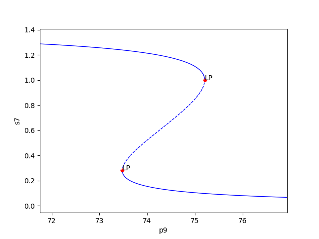
Similar to the mass conservation approach, we obtain multistability plots in the directory provided by the dir_path option in run_continuity_analysis (here it is the default value), where the plots follow the following format PCP (in terms of p as in the theory) _species id_index of params_for_global.png. The following is one multistability plot produced.
In addition to providing this more hands on approach to the numerical continuation routine, we also provide a greedy version of the numerical continuation routine. With this approach the user just needs to provide the species, parameters, and PCP. This routine does not guarantee that all multistability plots will be found, but it does provide a good place to start finding multistability plots. Once the greedy routine is ran, it is usually best to return to the more hands on approach described above. Note that as stated by the name, this approach is computationally greedy and will take a longer time than the more hands on approach. Below is the code used to run the greedy numerical continuation:
multistable_param_ind, plot_specifications = approach.run_greedy_continuity_analysis(species="s7", parameters=params_for_global_min,
                                                                                     auto_parameters={'PrincipalContinuationParameter': 're17'})

approach.generate_report()
This provides the following output:
Running continuity analysis ...
Elapsed time for continuity analysis in seconds: 534.1763272285461

Smallest value achieved by objective function: 0.0
76 point(s) passed the optimization criteria.
Number of multistability plots found: 73
Elements in params_for_global_min that produce multistability:
[0, 1, 2, 3, 4, 5, 6, 7, 8, 9, 10, 12, 13, 14, 15, 16, 17, 18, 19, 20, 21, 22, 23, 24, 25, 26, 27, 29, 30, 31, 32,
 33, 34, 35, 36, 37, 38, 39, 40, 41, 42, 43, 44, 45, 46, 47, 48, 49, 50, 51, 52, 53, 54, 55, 56, 57, 58, 59, 60,
 61, 62, 63, 64, 65, 67, 68, 69, 70, 71, 72, 73, 74, 75]
Note that some of these plots will be jagged or have missing sections in the plot. To produce better plots the hands on approach should be used.
For more examples of running the semi-diffusive approach please see Further Examples.